Profile a data frame

The package's single entry point. It runs type inference, missing-value analysis, summary statistics, normality tests, outlier detection, correlation analysis and a data-quality score, and (optionally) builds a set of ggplot2 visualisations. The result is a data_profile S3 object with print(), summary() and plot() methods.

Usage

profile_data(
  df,
  dataset_name = NULL,
  build_plots = TRUE,
  distributions = TRUE,
  normality = TRUE,
  outlier_method = "iqr",
  cor_method = c("pearson", "spearman"),
  group_by = NULL,
  verbose = FALSE
)

Arguments

df: A data frame with at least one row and one column and unique, non-empty column names.
dataset_name: Optional label stored in the metadata; defaults to the deparsed name of df.
build_plots: Whether to build the ggplot2 objects. Set FALSE to skip plotting on very wide data. Default TRUE.
distributions: Whether to build a per-column distribution plot (the eager, heaviest part of plotting). Set FALSE on wide data and use plot_distribution() on demand. Ignored if build_plots = FALSE. Default TRUE.
normality: Whether to run normality tests. Default TRUE.
outlier_method: Method passed to outlier_summary(): "iqr", "zscore" or "robust". Default "iqr".
cor_method: Correlation methods: any of "pearson", "spearman".
group_by: Optional name of a categorical column. If supplied, a grouped comparison of the numeric columns is added to the diagnostics (see compare_groups()).
verbose: Print progress messages. Default FALSE.

Value

An object of class data_profile: a list with elements metadata, statistics, diagnostics, plots and call.

Examples

p <- profile_data(iris)
p
#> <data_profile>
#>   dataset : iris
#>   size    : 150 rows x 5 columns
#>   types   : categorical=1, numeric=4
#>   missing : 0.0% of cells; 100.0% of rows complete
#>   quality : 99.7 / 100 (grade A)
#>   use summary() for details and plot() for figures.
summary(p)
#> Data profile for 'iris' (150 x 5), quality 99.7 (A)
#> 
#> -- numeric summary --
#>        column   n n_missing  mean    sd variance min  q1 median  q3 max iqr
#>  Sepal.Length 150         0 5.843 0.828    0.686 4.3 5.1   5.80 6.4 7.9 1.3
#>   Sepal.Width 150         0 3.057 0.436    0.190 2.0 2.8   3.00 3.3 4.4 0.5
#>  Petal.Length 150         0 3.758 1.765    3.116 1.0 1.6   4.35 5.1 6.9 3.5
#>   Petal.Width 150         0 1.199 0.762    0.581 0.1 0.3   1.30 1.8 2.5 1.5
#>  skewness kurtosis
#>     0.312   -0.574
#>     0.316    0.181
#>    -0.272   -1.396
#>    -0.102   -1.336
#> 
#> -- normality (Shapiro-Wilk) --
#>        column n_used shapiro_p normal
#>  Sepal.Length    150  1.02e-02  FALSE
#>   Sepal.Width    150  1.01e-01   TRUE
#>  Petal.Length    150  7.41e-10  FALSE
#>   Petal.Width    150  1.68e-08  FALSE
#> 
#> -- outliers (iqr) --
#>        column n_outliers  pct
#>  Sepal.Length          0 0.00
#>   Sepal.Width          4 2.67
#>  Petal.Length          0 0.00
#>   Petal.Width          0 0.00
#> 
#> -- strongest correlations (pearson) --
#>          var1         var2 correlation
#>  Petal.Length  Petal.Width       0.963
#>  Sepal.Length Petal.Length       0.872
#>  Sepal.Length  Petal.Width       0.818
#>   Sepal.Width Petal.Length      -0.428
#>   Sepal.Width  Petal.Width      -0.366
#>  Sepal.Length  Sepal.Width      -0.118
#> 
# \donttest{
plot(p, which = "correlation")

# }

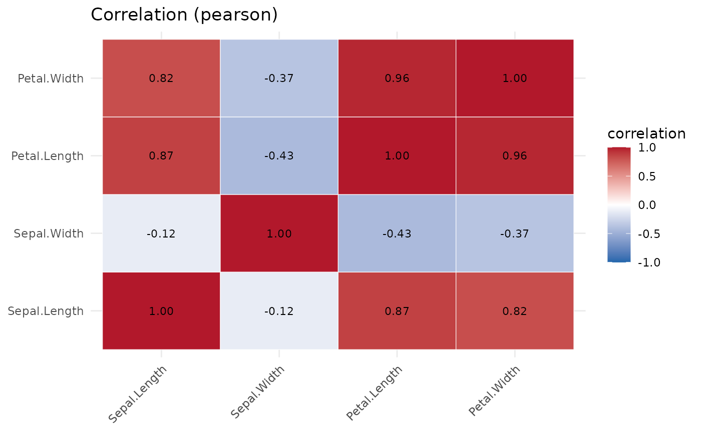Usage

Arguments

Value

See also

Examples