dataProfilerR turns a data frame into a structured
profile with one call: type inference, missing-value analysis, summary
statistics, normality tests, outlier detection, correlation, a
data-quality score, and ggplot2 figures.
A deliberately messy dataset
To show what the profiler surfaces, here is a small frame with missing values, an outlier, a constant column, and a high-cardinality text column.
set.seed(1)
n <- 200
df <- data.frame(
  age        = round(rnorm(n, 40, 12)),
  income     = c(rlnorm(n - 1, log(50000), 0.4), 5e6),   # one extreme outlier
  signup     = as.Date("2025-01-01") + sample(0:600, n, replace = TRUE),
  plan       = sample(c("free", "pro", "enterprise"), n, replace = TRUE),
  region     = sample(c("NA", "EU", "APAC"), n, replace = TRUE),
  constant   = 1L,                                        # zero-variance column
  note       = replicate(n, paste(sample(letters, 12), collapse = "")),
  stringsAsFactors = FALSE
)
df$income[sample(n, 20)] <- NA          # inject missingness
df$plan[sample(n, 8)]    <- NA
One call to profile it
p <- profile_data(df, dataset_name = "customers")
#> Warning in stats::cor(num_df, use = "pairwise.complete.obs", method = m): the
#> standard deviation is zero
#> Warning in stats::cor(num_df, use = "pairwise.complete.obs", method = m): the
#> standard deviation is zero
#> Warning in stats::cor(num_df, use = "pairwise.complete.obs", method = m): the
#> standard deviation is zero
#> Warning in stats::cor(num_df, use = "pairwise.complete.obs", method = m): the
#> standard deviation is zero
p
#> <data_profile>
#>   dataset : customers
#>   size    : 200 rows x 7 columns
#>   types   : categorical=2, date=1, integer=1, numeric=2, text=1
#>   missing : 2.0% of cells; 86.5% of rows complete
#>   quality : 96.2 / 100 (grade A)
#>   most missing: income (10.0%), plan (4.0%)
#>   use summary() for details and plot() for figures.
print() gives the headline: dimensions, type breakdown,
missingness, and the quality score. Note the score is below 100 – the
missingness and the constant column both cost points.
Drilling in with summary()
summary(p)
#> Data profile for 'customers' (200 x 7), quality 96.2 (A)
#>
#> -- numeric summary --
#>    column   n n_missing      mean        sd     variance      min       q1
#>       age 200         0    40.385     11.15 1.243180e+02    13.00    33.00
#>    income 180        20 82158.549 369253.45 1.363481e+11 15743.93 40392.28
#>  constant 200         0     1.000      0.00 0.000000e+00     1.00     1.00
#>    median       q3     max      iqr skewness kurtosis
#>     39.00    47.00      69    14.00    0.190   -0.199
#>  50065.35 67074.75 5000000 26682.47   13.233  173.753
#>      1.00     1.00       1     0.00       NA       NA
#>
#> -- columns with missing values --
#>  column n_missing pct_missing
#>  income        20          10
#>    plan         8           4
#>
#> -- normality (Shapiro-Wilk) --
#>    column n_used shapiro_p normal
#>       age    200  3.93e-01   TRUE
#>    income    180  9.16e-29  FALSE
#>  constant    200        NA  FALSE
#>
#> -- outliers (iqr) --
#>    column n_outliers  pct
#>       age          1 0.50
#>    income          4 2.22
#>  constant          0 0.00
#>
#> -- strongest correlations (pearson) --
#>    var1     var2 correlation
#>     age   income      -0.035
#>     age constant          NA
#>  income constant          NA
#>
#> -- date columns --
#>  column   n n_missing        min        max range_days n_unique max_gap_days
#>  signup 200         0 2025-01-03 2026-08-24        598      167           16
#>
#> -- categorical association (Cramer's V) --
#>        plan region
#> plan   1.00   0.02
#> region 0.02   1.00
The numeric summary shows income is heavily right-skewed
(large positive skewness and kurtosis) thanks to the injected outlier,
and the outlier table flags it. age looks roughly
symmetric.
The object is just a list
Everything is accessible directly, which makes the profile easy to use programmatically:
p$metadata$column_types
#>           age        income        signup          plan        region
#>     "numeric"     "numeric"        "date" "categorical" "categorical"
#>      constant          note
#>     "integer"        "text"
p$diagnostics$quality$components
#> completeness   uniqueness  variability  cleanliness
#>         98.0        100.0         85.7         99.1
head(p$statistics$numeric[, c("column", "mean", "sd", "skewness")])
#>     column      mean           sd   skewness
#> 1      age    40.385     11.14981  0.1904266
#> 2   income 82158.549 369253.44951 13.2334718
#> 3 constant     1.000      0.00000         NA
Figures
The figures are built during profile_data() and
retrieved with plot().
plot(p, which = "missing")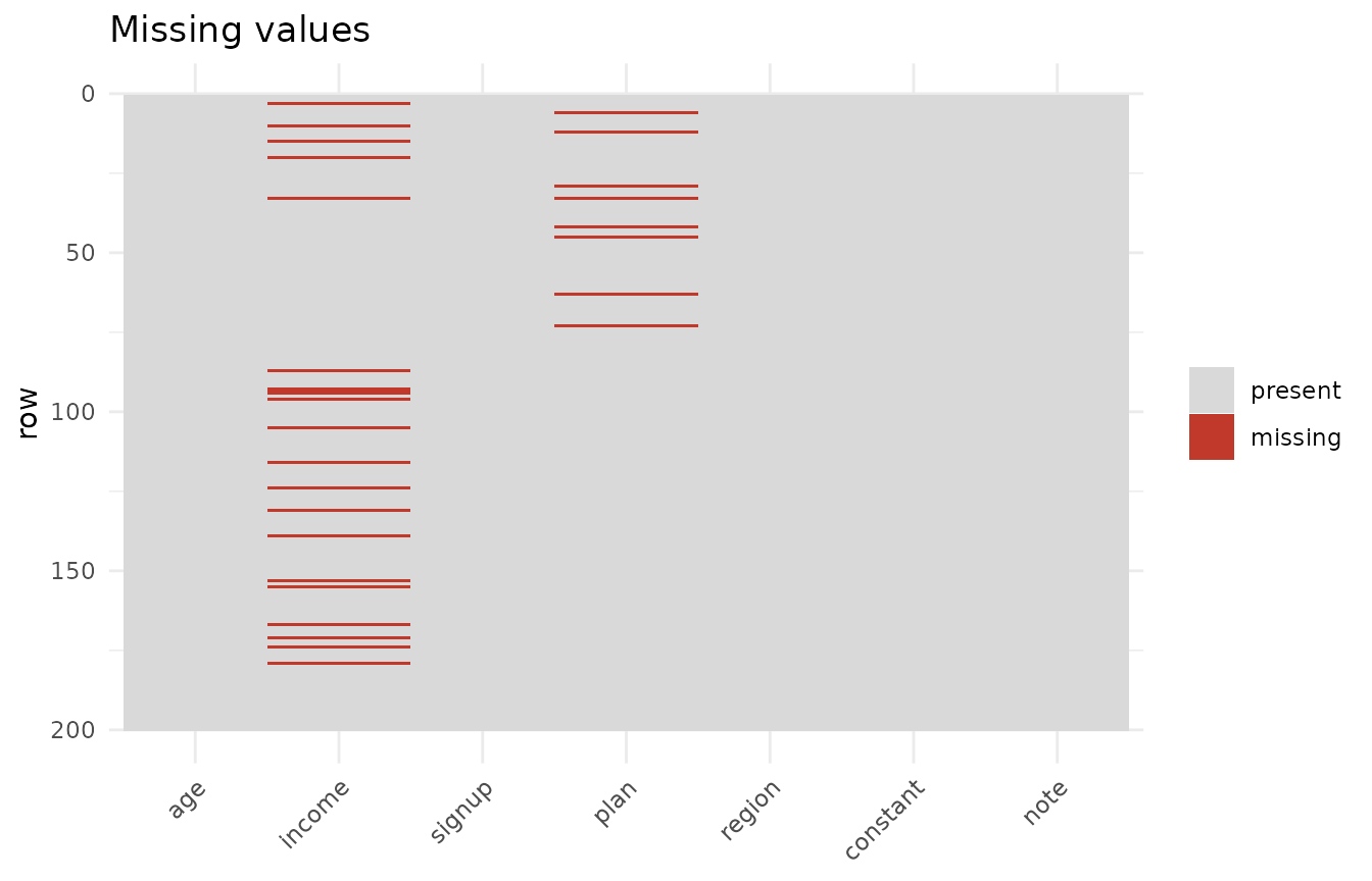
plot(p, which = "distribution", column = "income")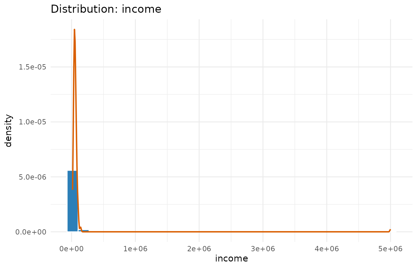
plot(p, which = "correlation")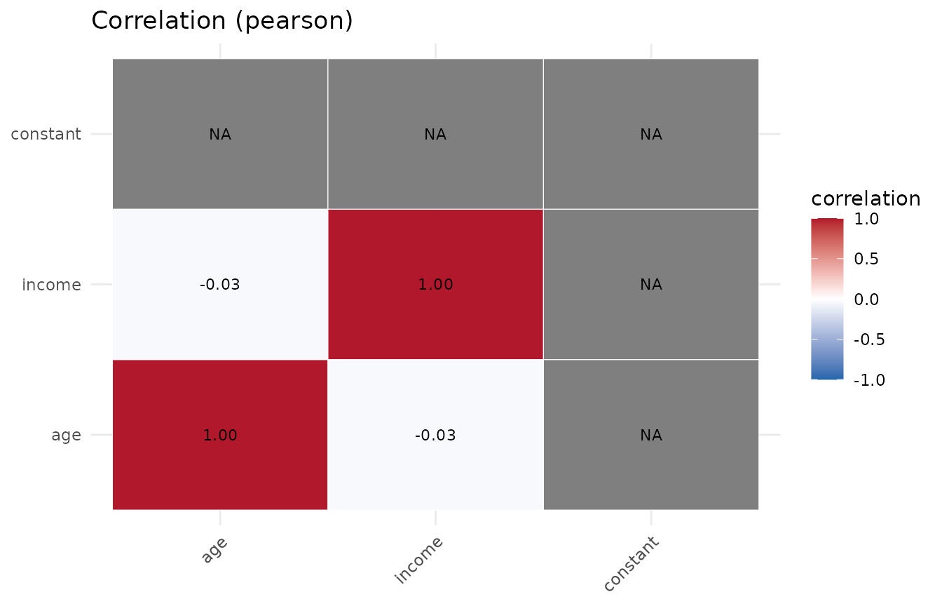
You can also call the plotting functions directly without a full
profile, e.g. plot_boxplots(df) or
plot_pairs(df, c("age", "income")).
Tuning the run
-
build_plots = FALSEskips figure construction on very wide data. -
outlier_methodcan be"iqr"(default),"zscore", or"robust"(median/MAD). -
cor_methodaccepts"pearson","spearman", or both. -
normality = FALSEskips the Shapiro-Wilk / Anderson-Darling tests.
p2 <- profile_data(df, build_plots = FALSE, outlier_method = "robust",
                   cor_method = "spearman")
#> Warning in stats::cor(num_df, use = "pairwise.complete.obs", method = m): the
#> standard deviation is zero
#> Warning in stats::cor(num_df, use = "pairwise.complete.obs", method = m): the
#> standard deviation is zero
#> Warning in stats::cor(num_df, use = "pairwise.complete.obs", method = m): the
#> standard deviation is zero
p2$diagnostics$outliers$per_column
#>     column n_outliers  pct
#> 1      age          0 0.00
#> 2   income          3 1.67
#> 3 constant          0 0.00
Beyond correlation (0.2.0)
Categorical columns get their own association matrix (Cramer’s V):
p$statistics$association
#>              plan     region
#> plan   1.00000000 0.02227124
#> region 0.02227124 1.00000000
plot(p, which = "association")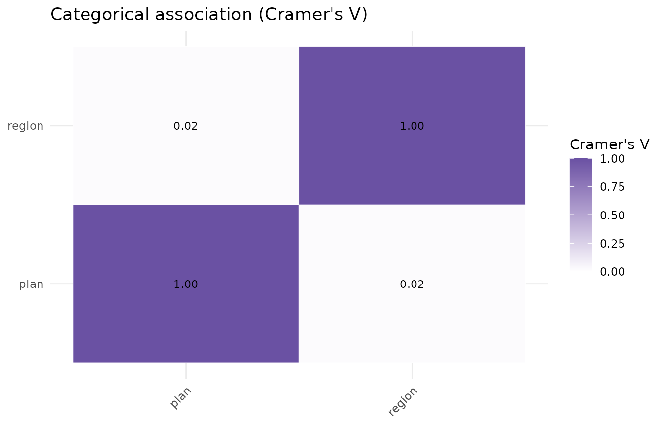
Date columns are profiled for range and gaps:
p$diagnostics$dates
#>   column   n n_missing        min        max range_days n_unique max_gap_days
#> 1 signup 200         0 2025-01-03 2026-08-24        598      167           16
And you can compare the numeric columns across the levels of a factor:
pg <- profile_data(df, group_by = "plan")
#> Warning in stats::cor(num_df, use = "pairwise.complete.obs", method = m): the
#> standard deviation is zero
#> Warning in stats::cor(num_df, use = "pairwise.complete.obs", method = m): the
#> standard deviation is zero
#> Warning in stats::cor(num_df, use = "pairwise.complete.obs", method = m): the
#> standard deviation is zero
#> Warning in stats::cor(num_df, use = "pairwise.complete.obs", method = m): the
#> standard deviation is zero
head(pg$diagnostics$groups$numeric_by_group, 8)
#>        group   column  n n_missing         mean           sd   median
#> 1 enterprise      age 70         0     40.87143     11.82103    40.50
#> 2 enterprise   income 63         7  53494.38196  20892.25942 49893.23
#> 3 enterprise constant 70         0      1.00000      0.00000     1.00
#> 4       free      age 59         0     40.16949     11.88907    40.00
#> 5       free   income 54         5  56576.18404  21851.55117 52620.50
#> 6       free constant 59         0      1.00000      0.00000     1.00
#> 7        pro      age 63         0     40.12698     10.23985    39.00
#> 8        pro   income 56         7 140692.97488 661501.68118 47833.91