Genomic REML without forming the covariance matrix

Heritability estimation and genomic prediction rest on the linear mixed model $$y = X\beta + g + e, \qquad g \sim N(0, \sigma^2_g G), \qquad e \sim N(0, \sigma^2_e I),$$ where $G$ is the genomic relationship matrix among $n$ individuals. Its variance components are estimated by restricted maximum likelihood (REML), usually with the average-information algorithm of Gilmour, Thompson and Cullis (1995). Every iteration of the exact algorithm factorizes $V = \sigma^2_g G + \sigma^2_e I$, which takes about $n^3/3$ operations, and holds several $n \times n$ matrices in memory. For 50,000 individuals each of those matrices takes 20 GB.

reml_sketch() runs the same algorithm but replaces every step that needs $V$ in full with a randomized one. This vignette explains how, checks the result against exact REML on data sets where both can be run, and measures how the two scale.

What an iteration needs

Write $P = V^{-1} - V^{-1}X(X^\top V^{-1}X)^{-1}X^\top V^{-1}$. The REML score is $$\frac{\partial \ell}{\partial \sigma^2_g} = -\tfrac12\{\mathrm{tr}(PG) - y^\top PGPy\}, \qquad \frac{\partial \ell}{\partial \sigma^2_e} = -\tfrac12\{\mathrm{tr}(P) - y^\top PPy\},$$ the average-information matrix is $$\mathrm{AI} = \tfrac12 \begin{pmatrix} y^\top PGPGPy & y^\top PGPPy \\ y^\top PPGPy & y^\top PPPy \end{pmatrix},$$ and each iteration moves $\theta = (\sigma^2_g, \sigma^2_e)$ to $\theta + \mathrm{AI}^{-1} \partial\ell/\partial\theta$. Apart from the two traces, everything is a product of $P$ with a vector, and a product with $P$ needs only solves with $V$. reml_sketch() obtains each piece as follows.

• Solves with $V$. The system $Vx = b$ is $(G + \mu I)x = b/\sigma^2_g$ with $\mu = \sigma^2_e/\sigma^2_g$. It is solved by conjugate gradients, preconditioned with a low-rank approximation of $G$ from rpchol() that is built once, before the first iteration. Only $\mu$ changes between iterations, and the preconditioner depends on $\mu$ only through a diagonal, so one approximation serves the whole fit.
• $\mathrm{tr}(PG)$. XTrace estimates it from products with $PG$, each of which costs one solve. The random test vectors are drawn once and reused at every iteration, so the iterations settle on a fixed point rather than wander with fresh noise.
• $\mathrm{tr}(P)$. $PV$ is a projection of rank $n - \mathrm{rank}(X)$, so $\sigma^2_g\,\mathrm{tr}(PG) + \sigma^2_e\,\mathrm{tr}(P) = n - \mathrm{rank}(X)$ exactly, and the second trace follows from the first at no cost.

With the default of 40 products for the trace, an iteration solves 44 systems, advanced together in five blocks by the block conjugate gradient solver behind pcg(). Each step then multiplies $G$ by a block of vectors. With $G$ held as a matrix that costs $O(n^2)$ per vector; given as grm_matrix(M) for an $n \times p$ genotype matrix $M$ it costs $O(np)$, and $G$ is never formed.

A worked example

Simulated genotypes for 1,500 individuals from four subpopulations, on 3,000 markers, with a trait of heritability 0.5:

library(matsketch)
set.seed(11)
dat <- sim_genomic(n = 1500, p = 3000, h2 = 0.5, pops = 4)
G <- grm_matrix(dat$M)
fit <- reml_sketch(dat$y, G)
fit
#> <reml_sketch> converged in 4 iterations (rpchol rank-100 preconditioner, XTrace with 40 products)
#>          estimate std.error
#> genetic    0.5212    0.0546
#> residual   0.4375    0.0404
#> h2         0.5436    0.0454
#>   linear systems solved : 180 (mean 8.4 CG iterations)

The history records each iteration’s estimates, the trace estimate, and the standard error of that trace estimate, which measures how far the randomized fit can sit from the exact one:

fit$history
#>   iteration   genetic  residual trace_PG trace_se       change
#> 1         1 0.5248868 0.4325594 1302.709 4.328189 1.187296e-01
#> 2         2 0.5211177 0.4375674 1333.567 4.193366 1.157773e-02
#> 3         3 0.5212062 0.4375185 1331.921 4.211137 1.698354e-04
#> 4         4 0.5212044 0.4375233 1331.864 4.210621 1.093405e-05
plot(fit)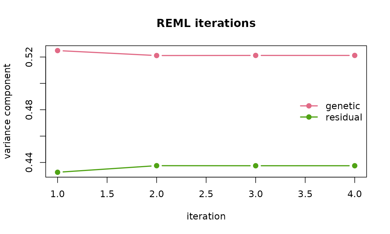

The exact fit, for comparison:

exact <- reml_exact(dat$y, as.matrix(G))
rbind(sketched = c(fit$sigma2, h2 = fit$h2, se_h2 = fit$se[["h2"]]),
      exact = c(exact$sigma2, h2 = exact$h2, se_h2 = exact$se[["h2"]]))
#>            genetic  residual        h2      se_h2
#> sketched 0.5212044 0.4375233 0.5436418 0.04541329
#> exact    0.5279405 0.4326637 0.5495922 0.04517044

The two estimates of $h^2$ differ by 0.13 exact standard errors: the error the sketch adds is small next to the sampling error of REML itself.

Each solve took 8.4 conjugate gradient iterations on average. The spectrum of $G$ shows why so few are needed:

ev <- eigen(as.matrix(G), symmetric = TRUE, only.values = TRUE)$values
mu <- fit$sigma2[["residual"]] / fit$sigma2[["genetic"]]
keep <- ev > 1e-8
plot(which(keep), ev[keep], log = "y", pch = 19, cex = 0.4, col = "#0072B2",
     xlab = "index", ylab = "eigenvalue of G")
abline(v = 100.5, lty = 2, col = "grey50")
abline(h = mu, lty = 3, lwd = 2, col = "#D55E00")
legend("topright", c("preconditioner rank", "mu at the estimate"),
       lty = c(2, 3), lwd = c(1, 2), col = c("grey50", "#D55E00"),
       bty = "n")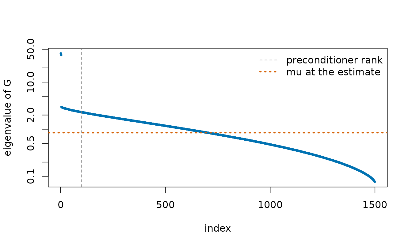

Population structure puts 3 eigenvalues far above the rest, and those are what the rank-100 preconditioner removes. An ideal rank-100 preconditioner maps the top 100 eigenvalues of $G + \mu I$ to $\lambda_{100} + \mu$ and leaves the others alone, so the preconditioned system has condition number at most about $(\lambda_{100} + \mu)/\mu = 3.7$, here with $\mu = 0.84$. At that condition number conjugate gradients need only a few iterations.

Accuracy over many data sets

The package ships the results of fitting 40 simulated data sets both ways, each with 2,000 individuals from four subpopulations, 4,000 markers and a true heritability of 0.3 or 0.6, all with the default settings of reml_sketch(). The script that produced them is data-raw/reml-benchmark.R in the package’s GitHub repository.

acc <- read.csv(system.file("extdata", "reml-accuracy.csv",
                            package = "matsketch"))
z <- (acc$sketch_h2 - acc$exact_h2) / acc$exact_se
summary(z)
#>     Min.  1st Qu.   Median     Mean  3rd Qu.     Max. 
#> -0.58182 -0.18397 -0.06672 -0.04044  0.12833  0.38212

op <- par(mfrow = c(1, 2), mar = c(4.2, 4.2, 1, 1))
cols <- ifelse(acc$true_h2 < 0.5, "#0072B2", "#D55E00")
plot(acc$exact_h2, acc$sketch_h2, pch = 19, col = cols, asp = 1,
     xlab = "exact REML estimate", ylab = "sketched REML estimate")
abline(0, 1, lty = 2)
legend("topleft", c("true h2 = 0.3", "true h2 = 0.6"), pch = 19,
       col = c("#0072B2", "#D55E00"), bty = "n")
hist(z, breaks = 12, col = "grey80", border = "white", main = "",
     xlab = "(sketched - exact) / exact SE")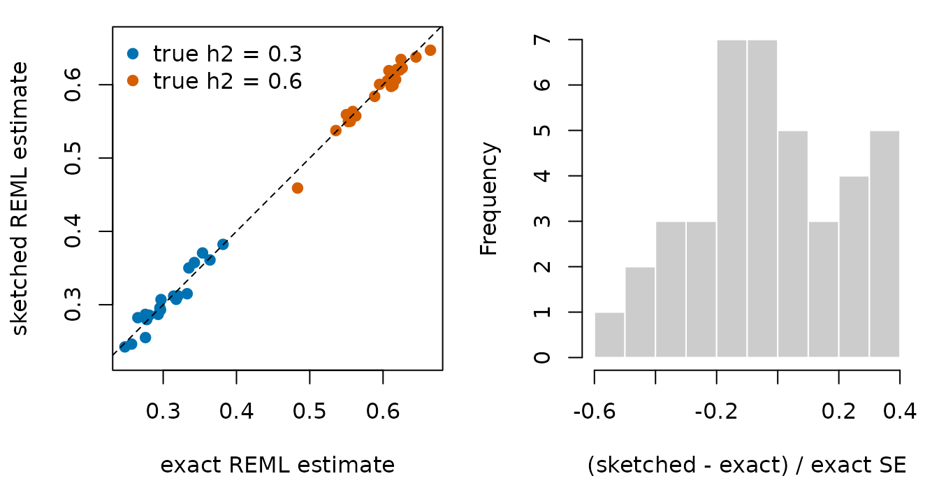

par(op)

Across the 40 data sets the sketched estimate was never more than 0.58 exact standard errors from the exact one, and the median difference was 0.16 standard errors. Measured against the true heritability, the root-mean-square error was 0.04 for exact REML and 0.042 for the sketch.

Scaling

The same script timed each fit as the number of individuals grew from 1,000 to 16,000, with 5,000 markers throughout. form_G is the time to build $G$ from the genotypes, which the exact fit and the dense sketched fit both need first. eigen is one eigendecomposition of $G$, the first step of exact methods that diagonalize $G$ once, such as FaST-LMM (Lippert et al., 2011); it was run up to 4,000 individuals.

sc <- read.csv(system.file("extdata", "reml-scaling.csv",
                           package = "matsketch"))
secs <- with(sc, tapply(seconds, list(n, method), sum))
secs <- secs[, c("form_G", "exact", "eigen", "sketch_dense", "sketch_lazy")]
round(secs, 1)
#>       form_G exact eigen sketch_dense sketch_lazy
#> 1000     2.8   1.6   0.7          1.2        10.1
#> 2000    11.8  12.0   6.0          4.2        20.9
#> 4000    48.3 114.9  49.2         17.8        48.8
#> 8000   193.0 848.1    NA         69.5        96.1
#> 16000     NA    NA    NA           NA       251.9

The plot adds the time to form $G$ to every method that needs it:

tot <- cbind(
  `exact REML` = secs[, "form_G"] + secs[, "exact"],
  `eigendecomposition only` = secs[, "form_G"] + secs[, "eigen"],
  `sketch, G formed` = secs[, "form_G"] + secs[, "sketch_dense"],
  `sketch, grm_matrix()` = secs[, "sketch_lazy"]
)
n <- as.numeric(rownames(secs))
cols <- c("#999999", "#0072B2", "#E69F00", "#D55E00")
matplot(n, tot / 60, log = "xy", type = "b", pch = 19, lty = 1, lwd = 2,
        col = cols, xlab = "individuals", ylab = "minutes")
legend("topleft", colnames(tot), col = cols, lwd = 2, pch = 19, bty = "n")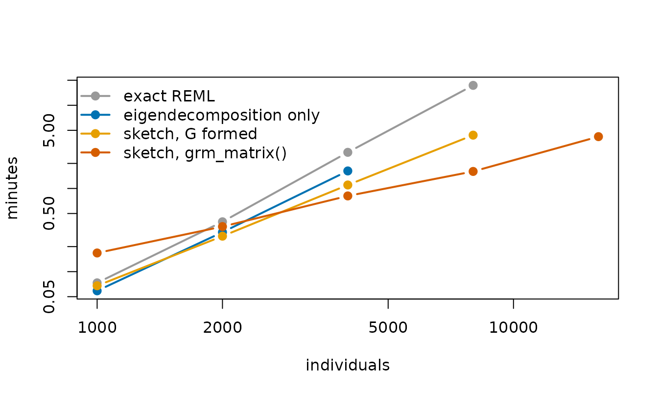

Exact REML took 7.4 times as long for 8,000 individuals as for 4,000, close to the eightfold its cubic cost predicts; including the time to form $G$ it took 17 minutes. The sketched fit on grm_matrix() took 1.6 minutes at that size, and 4.2 minutes for 16,000 individuals, where the exact fit was not attempted.

When $G$ is already in memory, the dense sketched fit is the fastest option from 2,000 individuals up; forming $G$ is the expensive part, and for 8,000 individuals it took longer than the dense sketched fit itself. A product with grm_matrix() costs about $2np$ operations against $n^2$ for a formed $G$, so with 5,000 markers it is the slower of the two per product until $n$ reaches 10,000. It pays for itself by skipping the formation of $G$ and its $n^2$ memory.

Memory is the other constraint. The exact fit holds about four $n \times n$ matrices, the dense sketched fit one, and the fit on grm_matrix() only the $n \times p$ genotypes. In gigabytes:

mem <- with(sc[sc$method %in% c("exact", "sketch_dense", "sketch_lazy"), ],
            tapply(memory_gb, list(n, method), sum))
round(mem, 2)
#>       exact sketch_dense sketch_lazy
#> 1000   0.03         0.01        0.04
#> 2000   0.12         0.03        0.07
#> 4000   0.48         0.12        0.15
#> 8000   1.91         0.48        0.30
#> 16000    NA           NA        0.60

At 16,000 individuals, four $n \times n$ matrices would take 7.6 GB.

Choosing the settings

• rank affects only speed. The preconditioner changes how many conjugate gradient iterations a solve takes, not what it converges to. The printed fit reports the mean iterations per solve; if that number is large, a larger rank will help.
• m sets the size of the randomized error, shown as trace_se in the history. It shrinks roughly like $1/\sqrt{m}$, and each extra product costs one more solve per iteration.
• estimator = "hutchinson" is available for comparison. The two estimators behave similarly when $G$ has no dominant eigenvalues, and XTrace is far more accurate when it does.
• cg_tol controls the accuracy of each solve. The default of $10^{-6}$ keeps its effect well below that of the randomized trace.

Limitations

reml_sketch() fits one relationship matrix plus a residual, for a Gaussian trait with no missing values. For a few thousand individuals the exact fit is fast and should be preferred. For a single relationship matrix, exact REML can also be computed after one eigendecomposition of $G$, which costs $O(n^3)$ time once and $O(n^2)$ memory; the sketched fit needs neither. Stochastic traces and conjugate gradients are the backbone of large-scale REML in animal breeding (Matilainen et al., 2013) and human genetics (Loh et al., 2015); reml_sketch() pairs them with the XTrace estimator and a randomly pivoted Cholesky preconditioner.

The timings above come from R 4.6.1 with its reference BLAS on one core of a Windows laptop. An optimized BLAS speeds up both kinds of fit.

References

Epperly, E. N., Tropp, J. A. and Webber, R. J. (2024). XTrace: making the most of every sample in stochastic trace estimation. SIAM Journal on Matrix Analysis and Applications 45, 1–23. doi:10.1137/23m1548323

Frangella, Z., Tropp, J. A. and Udell, M. (2023). Randomized Nyström preconditioning. SIAM Journal on Matrix Analysis and Applications 44, 718–752. doi:10.1137/21m1466244

Gilmour, A. R., Thompson, R. and Cullis, B. R. (1995). Average information REML: an efficient algorithm for variance parameter estimation in linear mixed models. Biometrics 51, 1440–1450. doi:10.2307/2533274

Lippert, C., Listgarten, J., Liu, Y., Kadie, C. M., Davidson, R. I. and Heckerman, D. (2011). FaST linear mixed models for genome-wide association studies. Nature Methods 8, 833–835. doi:10.1038/nmeth.1681

Loh, P.-R., Bhatia, G., Gusev, A., Finucane, H. K., Bulik-Sullivan, B. K. et al. (2015). Contrasting genetic architectures of schizophrenia and other complex diseases using fast variance-components analysis. Nature Genetics 47, 1385–1392. doi:10.1038/ng.3431

Matilainen, K., Mäntysaari, E. A., Lidauer, M. H., Strandén, I. and Thompson, R. (2013). Employing a Monte Carlo algorithm in Newton-type methods for restricted maximum likelihood estimation of genetic parameters. PLoS ONE 8, e80821. doi:10.1371/journal.pone.0080821

VanRaden, P. M. (2008). Efficient methods to compute genomic predictions. Journal of Dairy Science 91, 4414–4423. doi:10.3168/jds.2007-0980